Boundary Conditions

This section covers the different boundary conditions (BCs) implemented in VCAMS.

Although the goal of the software is creation of structures, the usefulness of creating BCs along with the model and the complexity of various BCs calls for implementation of various BCs in VCAMS. Definition of BCs for a part is not mandatory, and their accuracy/correctness is not guaranteed, so users are advised to check the theory, created BCs, and analysis results for possible errors.

Currently, three possible options are available regarding BCs:

• No boundary conditions

• Node Sets Only

• Linear Displacement Boundary Conditions

• Periodic Boundary Conditions

No Boundary Conditions

For this option, The user doesn’t need to do anything. The default state of a VoxelPart instance contains an empty BC definition. and in the GUI this option is selected by default.

Node Sets Only

This option creates node sets from the faces, edges, and vertices as shown in Fig. 10. These sets are exclusive, meaning for example that a face does not include the edges or vertices connected to it. Optionally, the user can create a set of simplified sets which only covers faces. Each of the explicit or simplified node set configurations are useful for a different kind of boundary conditions.

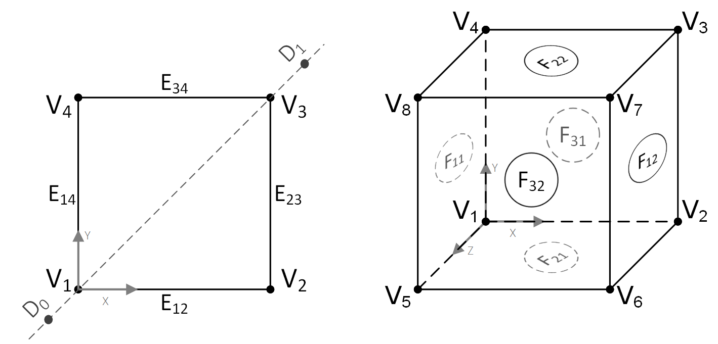
Fig. 10 Naming convention for faces, edges, and vertices in a cubic model.

Each square or cube has a number of vertices, which are named as shown in Fig. 10. Edges are numbered based on the vertices, e.g., E34 connects V3 and V4 with the numbers written in increasing order. In a cube, there are six faces. For face Fij, the number i refers to the direction, and j is the number of the face.

The program also uses a number of Dummy Nodes, which are known in Abaqus™ as Reference Points and are used for applying the actual BCs. These and are placed along the diagonal and offset from the end points. D₀ is always present and must be fixed in space to prevent rigid body motion and one or more D_i are used in equations that implement the desired BC.

Example B-1 shows a part in which the node sets are created.

Linear Displacement Boundary Conditions

In this boundary condition, the faces or edges of the part undergo a uniform displacement such that the face or edge retains its shape as a line or a plane. Currently, the formulation is implemented only for normal loads.

Based on the notation in Fig. 10 dummy nodes D₀ and D₁ are used for preventing rigid body motion and applying displacement, respectively. Eq. (1) describes the applied constraints for the 2D and 3D cases. Note that \(u^i\) refers to the displacement in the \(i\) direction and 1, 2, and 3 are used instead of x, y, and z.

(1)\[\begin{split}\begin{align} \text{2D} \begin{cases} u_{E_{14}}^1 &= u_{D_0}^1 \\ u_{E_{12}}^2 &= u_{D_0}^2 \\ u_{E_{23}}^1 &= u_{D_1}^1 \\ u_{E_{34}}^2 &= u_{D_1}^2 \\ \end{cases} &&& \text{3D} \begin{cases} u_{F_{11}}^1 &= u_{D_0}^1 \\ u_{F_{21}}^2 &= u_{D_0}^2 \\ u_{F_{31}}^3 &= u_{D_0}^3 \\ u_{F_{12}}^1 &= u_{D_1}^1 \\ u_{F_{22}}^2 &= u_{D_1}^2 \\ u_{F_{32}}^3 &= u_{D_1}^3 \\ \end{cases} \end{align}\end{split}\]

The procedure for applying a linear displacement BC is demonstrated in Example B-2.

Periodic Boundary Conditions

In this BC, opposing edges and faces have identical displacements. Implementation of a PBC requires three dummy nodes and three equations for each node on the boundary. Assume the the size of the cubic model in the three directions to be \(L_1\), \(L_2\), and \(L_3\), respectively. Based on this paper [1], for DOF values of \(i=1, 2, 3\) we can write the general 3D equations as:

(2)\[\begin{split}\begin{align} \text{Faces}& \begin{cases} u_i^{F_{12}} - u_i^{F_{11}} - L_1 u_i^{D_1} = 0 \\ u_i^{F_{22}} - u_i^{F_{21}} - L_2 u_i^{D_2} = 0 \\ u_i^{F_{32}} - u_i^{F_{31}} - L_3 u_i^{D_3} = 0 \end{cases} \\[0.5ex] \text{Edges}& \begin{cases} u_i^{E_{78}} - u_i^{E_{12}} - L_2 u_i^{D_2} - L_3 u_i^{D_3} = 0 \\ u_i^{E_{56}} - u_i^{E_{34}} + L_2 u_i^{D_2} - L_3 u_i^{D_3} = 0 \\ u_i^{E_{37}} - u_i^{E_{15}} - L_1 u_i^{D_1} - L_2 u_i^{D_2} = 0 \\ u_i^{E_{26}} - u_i^{E_{48}} - L_1 u_i^{D_1} + L_2 u_i^{D_2} = 0 \\ u_i^{E_{67}} - u_i^{E_{14}} - L_1 u_i^{D_1} - L_3 u_i^{D_3} = 0 \\ u_i^{E_{23}} - u_i^{E_{58}} - L_1 u_i^{D_1} + L_3 u_i^{D_3} = 0 \end{cases} \\[0.5ex] \text{Vertices}& \begin{cases} u_i^{V_7} - u_i^{V_1} - L_1 u_i^{D_1} - L_2 u_i^{D_2} - L_3 u_i^{D_3} = 0 \\ u_i^{V_8} - u_i^{V_2} + L_1 u_i^{D_1} - L_2 u_i^{D_2} - L_3 u_i^{D_3} = 0 \\ u_i^{V_5} - u_i^{V_3} + L_1 u_i^{D_1} + L_2 u_i^{D_2} - L_3 u_i^{D_3} = 0 \\ u_i^{V_6} - u_i^{V_4} - L_1 u_i^{D_1} + L_2 u_i^{D_2} - L_3 u_i^{D_3} = 0 \end{cases} \end{align}\end{split}\]

For 2D models, these can be written as:

(3)\[\begin{split}\begin{align} \text{Edges}& \begin{cases} u_1^{E_{34}} - u_1^{E_{12}} = 0 \\ u_2^{E_{34}} - u_2^{E_{12}} - L_2 u_2^{D_2} = 0 \\ u_1^{E_{23}} - u_1^{E_{14}} - L_1 u_1^{D_1} = 0 \\ u_2^{E_{23}} - u_2^{E_{14}} = 0 \end{cases} \\[0.5ex] \text{Vertices}& \begin{cases} u_1^{V_3} - u_1^{V_1} - L_1 u_1^{D_1} - L_2 u_1^{D_2} = 0 \\ u_2^{V_3} - u_2^{V_1} - L_1 u_2^{D_1} - L_2 u_2^{D_2} = 0 \\ u_1^{V_4} - u_1^{V_2} + L_1 u_1^{D_1} - L_2 u_1^{D_2} = 0 \\ u_2^{V_4} - u_2^{V_2} + L_1 u_2^{D_1} - L_2 u_2^{D_2} = 0 \\ \end{cases} \end{align}\end{split}\]

In the above equations, there are three dummy nodes that are used for applying the loading. The dummy nodes are used as to represent the coarse scale deformation gradient as formulated in Ref [1]. Assuming that the deformation tensor \(\mathbf{U}\) is an input, Ref [1] shows that translations imposed on the dummy nodes must be:

(4)\[\mathbf{u}_i^{D_j} = \mathbf{U} - \delta_{ij}\]

or in matrix form:

(5)\[\begin{split}\begin{bmatrix} u_1^{D_1} & u_2^{D_1} & u_3^{D_1} \\ u_1^{D_2} & u_2^{D_2} & u_3^{D_2} \\ u_1^{D_3} & u_2^{D_3} & u_3^{D_3} \end{bmatrix} = \begin{bmatrix} U_{11} & U_{12} & U_{13} \\ U_{21} & U_{22} & U_{23} \\ U_{31} & U_{32} & U_{33} \end{bmatrix} - \mathbf{I} = \begin{bmatrix} U_{11} - 1 & U_{12} & U_{13} \\ U_{21} & U_{22} - 1 & U_{23} \\ U_{31} & U_{32} & U_{33} - 1 \end{bmatrix}\end{split}\]

The strain tensor is symmetric and it follows that the applied deformation must be symmetric. Therefore, we can simplify the previous equation and obtain the translation vectors of each dummy node:

(6)\[\begin{split}\begin{cases} \begin{alignat}{4} \vec{u}^{D_1} = (&U_{11} - 1&,&\ U_{12} &,&\ U_{13} &)& \\ \vec{u}^{D_2} = (&U_{12} &,&\ U_{22} - 1&,&\ U_{23} &)& \\ \vec{u}^{D_3} = (&U_{13} &,&\ U_{23} &,&\ U_{33} - 1&)& \end{alignat} \end{cases}\end{split}\]

It is evident from Eq. (6) that only six independent values are necessary for applying the actual loading to a periodic boundary condition. Additionally, in order to prevent rigid body motion, the vertex \(V_1\) must be fixed in space.

The procedure for applying a periodic BC is demonstrated in Example B-3. It is recommended that the users reproduce that example as an exercise.

[1] (1,2,3)

Walters, D. J., Luscher, D. J., Yeager, J. D. (2021). Considering computational speed vs. accuracy: Choosing appropriate mesoscale RVE boundary conditions. Computer Methods in Applied Mechanics and Engineering, 374, 113572. https://doi.org/10.1016/j.cma.2020.113572