Example G-9: 3D Part from Image Series
In this example, a 3D part is created based on an image series. This modeling method imports the images, applies a scale, and automatically thresholds it using the default Otsu’s method. There is also a noise removal option. Number of voxels and the base material are set automatically. This example mirrors Example C-6.
The image set used in this example is a micro-CT scan of the tibia of a mouse. It has been made available by the authors of this data paper [1] and its corresponding figshare collection. The dataset is large and has not been included here, but it can be downloaded from the aforementioned links.
In the collection, the micro-CT scan used is named MicroCT of mouse tibiae-oim4 and consists of 991 images (which will be in the z-direction of the model), each being 784×784 pixels. Each voxel is reported to be 5.06 micrometers. The model is scaled at 50%, which means that voxel size must doubled.
Here, we first select the Image Processing (Image Stack for 3D Part) from the Model Manipulations tab and then move to the Basic Model Information tab. This disables the number of voxels which is determined by the input image.
We want to model a three dimensional structure a voxel size of 0.01012 units in all directions and a base material of 0 (empty space). The image processing code will automatically set the other elements to 2. We set the parameter log_debug to True for demonstration purposes.
Afterwards, the parameters for image processing are entered in the Model Manipulations tab. The first parameter is Image Path String which is a path that describes all of the images in the sequence. They will be automatically be loaded in alphabetical order. Afterwards, we set the Scale and we can also request noise removal. The pixels selected by the image are automatically set to 2.
The part is then exported to an Abaqus™ input file in 3D mode with C3D8R elements. The Non-Empty elements are requested to be exported.
The following figures show the various tabs of the GUI in this example:
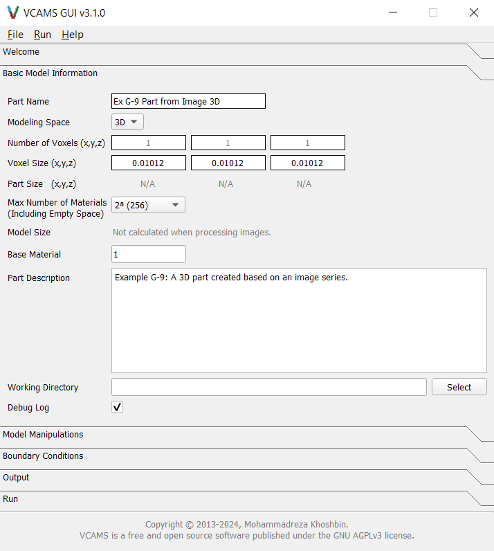
Fig. 65 The GUI’s “Basic Model Information” tab for Example G-9.
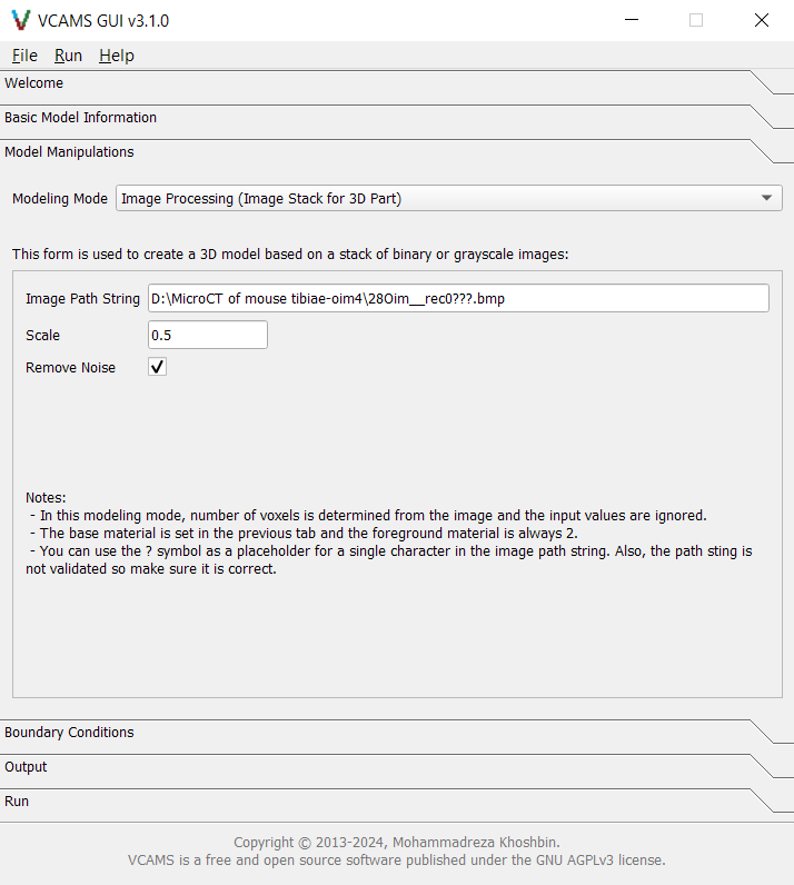
Fig. 66 The GUI’s “Model Manipulations” tab for Example G-9.
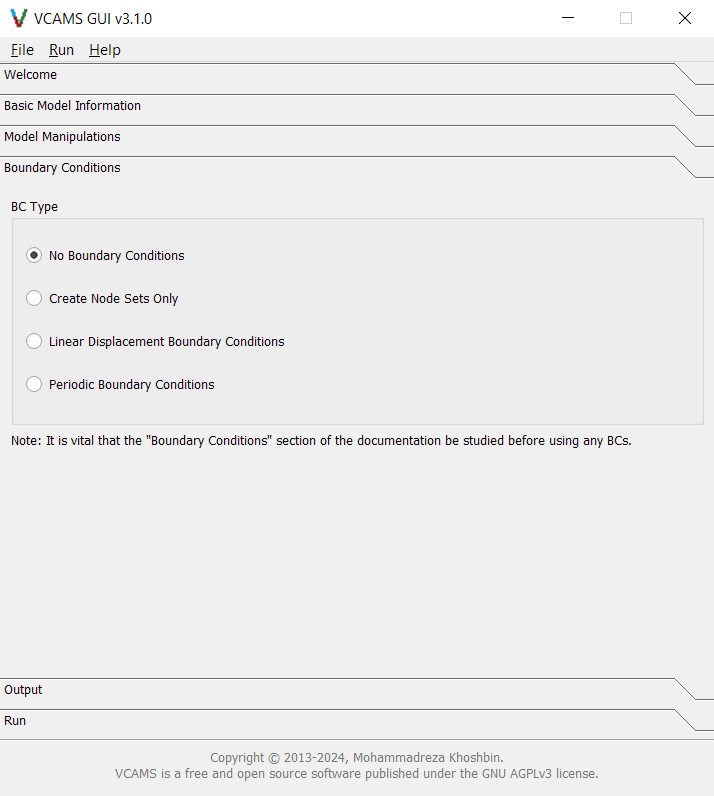
Fig. 67 The GUI’s “Boundary Conditions” tab for Example G-9.
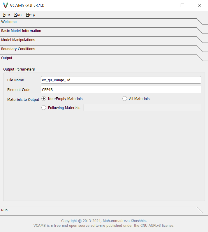
Fig. 68 The GUI’s “Output” tab for Example G-9.
After filling the form, the model can be created by pressing the “Create Model” button. The screen automatically switches to the Run tab and will show the program log.
At the end of the process, a dialog box announces the completion and gives the path to the output file.
Also, the program log and a summary of model information will be shown in the Process Log section of the Run tab. It will also be written to a .log file in the output folder.
Finally, a configuration file based on the examples will be written to the output folder
and can be used to import the model in the future.
It will look like this.