Example C-11: Dispersion of Shapes based on Volume Fraction
This example demonstrates the use of the ShapeDispersionArray class
for creating a Boolean mask which is then used to manipulate the part.
This example deals with the case when we want to achieve a specific volume fraction (VF).
Example C-10 deals with creating and dispersing a specific number of shapes.
A ShapeDispersionArray instance contains
a number of shape requests which are used to create and disperse shapes in it.
Using this class can be quite complicated and computationally expensive
An example is demonstrated in the 2D space.
First, a 2D part with a shape of 200×200 voxels is created with a base material of 1 and a voxel size of 0.005 units in all directions. The parameter log_debug is set to True for demonstration purposes:
part = VoxelPart(size=(200, 200), base_material=1,
                 voxel_size=(0.005, 0.005),
                 name='Ex C-11 Dispersion of Shapes with Specified VF',
                 description='A 2D square 200*200 part created with '
                             'a volume fraction of shapes randomly dispersed in it.',
                 log_debug=True)
At this point, we will define a few parameters that will be used in the future. The first, is the number of boundary pixels and subsequently, boundary length:
num_bound_pixels = 2
bound_length = num_bound_pixels * part.voxel_size[0]
And the second one is the minimum acceptable value for radius r that we can accept:
min_valid_r = 4 * part.voxel_size[0]
Now we can define a 2D ShapeDispersionArray in the 2D space based on the VoxelPart instance:
shape_disp_array_obj = ShapeDispersionArray(dim='2D', part=part,
                                            num_bound_pixels=num_bound_pixels,
                                            short_msg=True)
Then, two shape requests are added without specifying the number of shapes.
The first is a request instances of type Circle.
This is a 2D circle which requires the following:
Some values for the radius. Although they are random, we would like a normal distribution for them and since radius must be positive, we will use a truncated normal distribution. To do so, we create an instance of
TruncatedNormalDistributionDispersion. Number of values is not set (defaults to None), and mean and standard deviation are set to 0.05 and 0.02, respectively. bound_a is set to min_valid_r which ensures that values are greater than min_valid_r.A random value for the x coordinate. An instance of
RandomDispersionis created and used. The minimum value is 0, and the maximum value is the part’s size in the x direction. A boundary is defined, but unlike Example C-10, it is set to the bound_length parameter because we do not have any values for the radius so there is no maximum radius to be used. This helps but does not ensure that no circle is placed outside the ShapeDispersionArray instance.A random value for the y coordinate. See above.
We can now add a shape request for the circles:
circle_r = TruncatedNormalDistributionDispersion(target_mean=0.05, target_std=0.02, bound_a=min_valid_r)
circle_xc = RandomDispersion(0, part.real_size[0], bound_length)
circle_yc = RandomDispersion(0, part.real_size[1], bound_length)
shape_disp_array_obj.add_shape_request(num_shapes=None, cls=Circle,
                                       xc=circle_xc, yc=circle_yc, r=circle_r, br=bound_length)
The second shape request is for instances of type Ellipse.
This is done similar to the previous request:
ellipse_a = TruncatedNormalDistributionDispersion(target_mean=0.06, target_std=0.03, bound_a=min_valid_r)
ellipse_aspect_ratio = TruncatedNormalDistributionDispersion(target_mean=1, target_std=0.25, bound_a=0.1)
ellipse_xc = RandomDispersion(0, part.real_size[0])
ellipse_yc = RandomDispersion(0, part.real_size[1])
ellipse_alpha = RandomDispersion(low=0, high=360)
shape_disp_array_obj.add_shape_request(num_shapes=None, cls=EllipseFromAspectRatio,
                                       xc=ellipse_xc, yc=ellipse_yc, alpha=ellipse_alpha,
                                       a=ellipse_a, aspect_ratio=ellipse_aspect_ratio,
                                       ba=bound_length, bb=bound_length)
Now we can disperse the shapes in the ShapeDispersionArray instance.
Dispersion may or may not be successful based on the requests
and the specified number of trials and attempts.
This is even more difficult and error-prone than Example C-10.
See disperse_shapes()
for a list of parameters.
Here we want a volume fraction (VF) of 30% and assume that between 5 and 20 shapes (for each of the two requested shapes) is the correct answer. We will also attempt placement of each shape 100 times, try placing each set of shapes 1000 times, and regenerate the entire stack of shapes 100 times. Therefore, the command will be:
shape_disp_array_obj.disperse_shapes_vf(target_vf=0.30, vf_tolerance=0.03,
                                        min_num_shapes=5, max_num_shapes=20,
                                        max_attempts=100, max_trials=1000, max_generations=100)
If dispersion is successful, we can use resulting mask to manipulate the part. When using the ShapeDispersionArray class we don’t need to calculate a mask, we just ask it to give us its mask using the ShapeDispersionArray’s mask property which will always be up-to-date. This Boolean mask is applied to the part with a value of 2. This means that the values of the elements selected by the mask are set to 2:
part.apply_mask(mask=shape_array_obj.mask, value=2)
Finally, The part is exported to an Abaqus™ input file in 2D mode with CPE4R elements. The Non-Empty elements (which happens to be the whole model), are requested to be exported.
The code can be found in the examples folder of the main repository. It is also included below:
"""Script for Example C-11: Dispersion of Shapes based on Volume Fraction"""

from vcams.mask.shape import Circle, EllipseFromAspectRatio
from vcams.mask.shape_dispersion import ShapeDispersionArray, RandomDispersion, TruncatedNormalDistributionDispersion
from vcams.voxelpart import VoxelPart

# Create the part.
part = VoxelPart(size=(200, 200), base_material=1, voxel_size=(0.005, 0.005),
                 name='Ex C-11 Dispersion Shapes VF',
                 description='A 2D square 200*200 part created with '
                             'a volume fraction of shapes randomly dispersed in it.', log_debug=True)

# Set the number of boundary pixels and calculate the respective length.
num_bound_pixels = 2
bound_length = num_bound_pixels * part.voxel_size[0]

# Set the minimum value for radius used for truncating the random distributions.
min_valid_r = 4 * part.voxel_size[0]

# Create a ShapeArray based on the VoxelPart object.
shape_disp_array_obj = ShapeDispersionArray(dim='2D', part=part,
                                            num_bound_pixels=0, wrap_mask=True, short_msg=True)

# Request the circles.
# Note that the boundary for RandomDispersion instances
# is only set to bound_length because we do not have any values
# for the radius so there is no maximum radius to be added to it.
# This means that some circles may touch the boundary.
circle_r = TruncatedNormalDistributionDispersion(target_mean=0.05, target_std=0.02, bound_a=min_valid_r)
circle_xc = RandomDispersion(0, part.real_size[0], bound_length)
circle_yc = RandomDispersion(0, part.real_size[1], bound_length)
shape_disp_array_obj.add_shape_request(num_shapes=None, cls=Circle,
                                       xc=circle_xc, yc=circle_yc, r=circle_r, br=bound_length)

# Request the ellipses.
ellipse_a = TruncatedNormalDistributionDispersion(target_mean=0.06, target_std=0.03, bound_a=min_valid_r)
ellipse_aspect_ratio = TruncatedNormalDistributionDispersion(target_mean=1, target_std=0.25, bound_a=0.1)
ellipse_xc = RandomDispersion(0, part.real_size[0])
ellipse_yc = RandomDispersion(0, part.real_size[1])
ellipse_alpha = RandomDispersion(low=0, high=180)
shape_disp_array_obj.add_shape_request(num_shapes=None, cls=EllipseFromAspectRatio,
                                       xc=ellipse_xc, yc=ellipse_yc, alpha=ellipse_alpha,
                                       a=ellipse_a, aspect_ratio=ellipse_aspect_ratio,
                                       ba=bound_length, bb=bound_length)

# Disperse the shapes in shape_disp_array_obj with the desired target_vf.
shape_disp_array_obj.disperse_shapes_vf(target_vf=0.30, vf_tolerance=0.03,
                                        min_num_shapes=5, max_num_shapes=20,
                                        max_attempts=100, max_trials=1000, max_generations=100)

# Apply the Boolean mask to the part.
part.apply_mask(mask=shape_disp_array_obj.mask, value=2)

# # Output the part.
part.output_abaqus_inp(file_name='ex_c11_shape_dispersion_vf',
                       elem_code='CPE4R', dim='2D',
                       material_elem_sets='Non-Empty')
The final model looks like Fig. 26. Note that elements in different sets are shown in different colors.
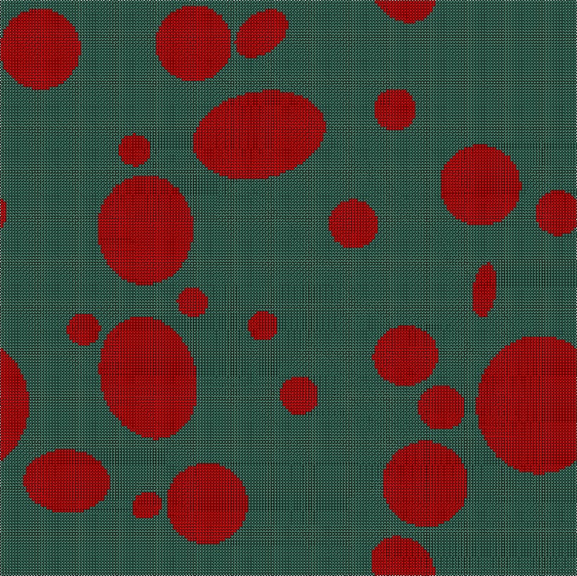
Fig. 26 Final model of Example C-11. Element sets corresponding to MAT-1 and MAT-2 are shown in green and red, respectively.